if (!require("pacman")) install.packages("pacman")Loading required package: pacmanpacman::p_load(terra, raster, mapview, dplyr, sf, lubridate, downloader)Handling raster data with terra
This is my practice sections following R as GIS for Economists.
if (!require("pacman")) install.packages("pacman")Loading required package: pacmanpacman::p_load(terra, raster, mapview, dplyr, sf, lubridate, downloader)(
IA_cdl_2015 <- raster::raster("Data/IA_cdl_2015.tif")
)class : RasterLayer
dimensions : 11671, 17795, 207685445 (nrow, ncol, ncell)
resolution : 30, 30 (x, y)
extent : -52095, 481755, 1938165, 2288295 (xmin, xmax, ymin, ymax)
crs : +proj=aea +lat_0=23 +lon_0=-96 +lat_1=29.5 +lat_2=45.5 +x_0=0 +y_0=0 +ellps=GRS80 +towgs84=0,0,0,0,0,0,0 +units=m +no_defs
source : IA_cdl_2015.tif
names : Layer_1
values : 0, 229 (min, max)IA_cdl_2016 <- raster::raster("Data/IA_CDL_2016.tif")
#--- stack the two ---#
(
IA_cdl_stack <- raster::stack(IA_cdl_2015, IA_cdl_2016)
)class : RasterStack
dimensions : 11671, 17795, 207685445, 2 (nrow, ncol, ncell, nlayers)
resolution : 30, 30 (x, y)
extent : -52095, 481755, 1938165, 2288295 (xmin, xmax, ymin, ymax)
crs : +proj=aea +lat_0=23 +lon_0=-96 +lat_1=29.5 +lat_2=45.5 +x_0=0 +y_0=0 +ellps=GRS80 +towgs84=0,0,0,0,0,0,0 +units=m +no_defs
names : Layer_1, IA_CDL_2016
min values : 0, 0
max values : 229, 241 # I am not evaluating this cell because it takes quite some time to execute.
#--- stack the two ---#
IA_cdl_brick <- brick(IA_cdl_stack)
#--- or this works as well ---#
# IA_cdl_brick <- brick(IA_cdl_2015, IA_cdl_2016)
#--- take a look ---#
IA_cdl_brick#--- convert to a SpatRaster ---#
IA_cdl_2015_sr <- terra::rast(IA_cdl_2015)
#--- convert to a SpatRaster ---#
IA_cdl_stack_sr <- terra::rast(IA_cdl_stack)Warning: [rast] CRS do not match#--- take a look ---#
IA_cdl_2015_srclass : SpatRaster
dimensions : 11671, 17795, 1 (nrow, ncol, nlyr)
resolution : 30, 30 (x, y)
extent : -52095, 481755, 1938165, 2288295 (xmin, xmax, ymin, ymax)
coord. ref. : +proj=aea +lat_0=23 +lon_0=-96 +lat_1=29.5 +lat_2=45.5 +x_0=0 +y_0=0 +ellps=GRS80 +towgs84=0,0,0,0,0,0,0 +units=m +no_defs
source : IA_cdl_2015.tif
name : Layer_1
min value : 0
max value : 229 # create a single-layer from multiple single-layer
IA_cdl_2016_sr <- terra::rast(IA_cdl_2016)
# concatenate
(
IA_cdl_ml_sr <- c(IA_cdl_2015_sr, IA_cdl_2016_sr)
)Warning: [rast] CRS do not matchclass : SpatRaster
dimensions : 11671, 17795, 2 (nrow, ncol, nlyr)
resolution : 30, 30 (x, y)
extent : -52095, 481755, 1938165, 2288295 (xmin, xmax, ymin, ymax)
coord. ref. : +proj=aea +lat_0=23 +lon_0=-96 +lat_1=29.5 +lat_2=45.5 +x_0=0 +y_0=0 +ellps=GRS80 +towgs84=0,0,0,0,0,0,0 +units=m +no_defs
sources : IA_cdl_2015.tif
IA_CDL_2016.tif
color table : 2
names : Layer_1, IA_CDL_2016
min values : 0, 0
max values : 229, 241 IA_cdl_stack_sr %>% raster::raster()class : RasterLayer
dimensions : 11671, 17795, 207685445 (nrow, ncol, ncell)
resolution : 30, 30 (x, y)
extent : -52095, 481755, 1938165, 2288295 (xmin, xmax, ymin, ymax)
crs : +proj=aea +lat_0=23 +lon_0=-96 +lat_1=29.5 +lat_2=45.5 +x_0=0 +y_0=0 +ellps=GRS80 +towgs84=0,0,0,0,0,0,0 +units=m +no_defs
source : IA_cdl_2015.tif
names : Layer_1
values : 0, 229 (min, max)# %>% raster::stack()
# %>% raster::brick() #--- Illinois county boundary ---#
(
IL_county <-
tigris::counties(
state = "Illinois",
progress_bar = FALSE
) %>%
dplyr::select(STATEFP, COUNTYFP)
)Retrieving data for the year 2022Simple feature collection with 102 features and 2 fields
Geometry type: MULTIPOLYGON
Dimension: XY
Bounding box: xmin: -91.51308 ymin: 36.9703 xmax: -87.01994 ymax: 42.50848
Geodetic CRS: NAD83
First 10 features:
STATEFP COUNTYFP geometry
86 17 067 MULTIPOLYGON (((-90.90609 4...
92 17 025 MULTIPOLYGON (((-88.69516 3...
131 17 185 MULTIPOLYGON (((-87.89243 3...
148 17 113 MULTIPOLYGON (((-88.91954 4...
158 17 005 MULTIPOLYGON (((-89.37207 3...
159 17 009 MULTIPOLYGON (((-90.53674 3...
213 17 083 MULTIPOLYGON (((-90.1459 39...
254 17 147 MULTIPOLYGON (((-88.46335 4...
266 17 151 MULTIPOLYGON (((-88.48289 3...
303 17 011 MULTIPOLYGON (((-89.16654 4...(
IL_county_sv <- terra::vect(IL_county)
) class : SpatVector
geometry : polygons
dimensions : 102, 2 (geometries, attributes)
extent : -91.51308, -87.01994, 36.9703, 42.50848 (xmin, xmax, ymin, ymax)
coord. ref. : lon/lat NAD83 (EPSG:4269)
names : STATEFP COUNTYFP
type : <chr> <chr>
values : 17 067
17 025
17 185(
IA_cdl_2015_sr <- terra::rast("Data/IA_cdl_2015.tif")
)class : SpatRaster
dimensions : 11671, 17795, 1 (nrow, ncol, nlyr)
resolution : 30, 30 (x, y)
extent : -52095, 481755, 1938165, 2288295 (xmin, xmax, ymin, ymax)
coord. ref. : +proj=aea +lat_0=23 +lon_0=-96 +lat_1=29.5 +lat_2=45.5 +x_0=0 +y_0=0 +ellps=GRS80 +towgs84=0,0,0,0,0,0,0 +units=m +no_defs
source : IA_cdl_2015.tif
name : Layer_1
min value : 0
max value : 229 #--- the list of path to the files ---#
files_list <- c("Data/IA_cdl_2015.tif", "Data/IA_CDL_2016.tif")
#--- read the two at the same time ---#
(
multi_layer_sr <- terra::rast(files_list)
)Warning: [rast] CRS do not matchclass : SpatRaster
dimensions : 11671, 17795, 2 (nrow, ncol, nlyr)
resolution : 30, 30 (x, y)
extent : -52095, 481755, 1938165, 2288295 (xmin, xmax, ymin, ymax)
coord. ref. : +proj=aea +lat_0=23 +lon_0=-96 +lat_1=29.5 +lat_2=45.5 +x_0=0 +y_0=0 +ellps=GRS80 +towgs84=0,0,0,0,0,0,0 +units=m +no_defs
sources : IA_cdl_2015.tif
IA_CDL_2016.tif
color table : 2
names : Layer_1, IA_CDL_2016
min values : 0, 0
max values : 229, 241 terra::crs(IA_cdl_2015_sr)[1] "BOUNDCRS[\n SOURCECRS[\n PROJCRS[\"unnamed\",\n BASEGEOGCRS[\"GRS 1980(IUGG, 1980)\",\n DATUM[\"unknown\",\n ELLIPSOID[\"GRS80\",6378137,298.257222101,\n LENGTHUNIT[\"metre\",1,\n ID[\"EPSG\",9001]]]],\n PRIMEM[\"Greenwich\",0,\n ANGLEUNIT[\"degree\",0.0174532925199433,\n ID[\"EPSG\",9122]]]],\n CONVERSION[\"Albers Equal Area\",\n METHOD[\"Albers Equal Area\",\n ID[\"EPSG\",9822]],\n PARAMETER[\"Latitude of false origin\",23,\n ANGLEUNIT[\"degree\",0.0174532925199433],\n ID[\"EPSG\",8821]],\n PARAMETER[\"Longitude of false origin\",-96,\n ANGLEUNIT[\"degree\",0.0174532925199433],\n ID[\"EPSG\",8822]],\n PARAMETER[\"Latitude of 1st standard parallel\",29.5,\n ANGLEUNIT[\"degree\",0.0174532925199433],\n ID[\"EPSG\",8823]],\n PARAMETER[\"Latitude of 2nd standard parallel\",45.5,\n ANGLEUNIT[\"degree\",0.0174532925199433],\n ID[\"EPSG\",8824]],\n PARAMETER[\"Easting at false origin\",0,\n LENGTHUNIT[\"metre\",1],\n ID[\"EPSG\",8826]],\n PARAMETER[\"Northing at false origin\",0,\n LENGTHUNIT[\"metre\",1],\n ID[\"EPSG\",8827]]],\n CS[Cartesian,2],\n AXIS[\"easting\",east,\n ORDER[1],\n LENGTHUNIT[\"metre\",1,\n ID[\"EPSG\",9001]]],\n AXIS[\"northing\",north,\n ORDER[2],\n LENGTHUNIT[\"metre\",1,\n ID[\"EPSG\",9001]]]]],\n TARGETCRS[\n GEOGCRS[\"WGS 84\",\n DATUM[\"World Geodetic System 1984\",\n ELLIPSOID[\"WGS 84\",6378137,298.257223563,\n LENGTHUNIT[\"metre\",1]]],\n PRIMEM[\"Greenwich\",0,\n ANGLEUNIT[\"degree\",0.0174532925199433]],\n CS[ellipsoidal,2],\n AXIS[\"geodetic latitude (Lat)\",north,\n ORDER[1],\n ANGLEUNIT[\"degree\",0.0174532925199433]],\n AXIS[\"geodetic longitude (Lon)\",east,\n ORDER[2],\n ANGLEUNIT[\"degree\",0.0174532925199433]],\n USAGE[\n SCOPE[\"Horizontal component of 3D system.\"],\n AREA[\"World.\"],\n BBOX[-90,-180,90,180]],\n ID[\"EPSG\",4326]]],\n ABRIDGEDTRANSFORMATION[\"Transformation to WGS84\",\n METHOD[\"Position Vector transformation (geog2D domain)\",\n ID[\"EPSG\",9606]],\n PARAMETER[\"X-axis translation\",0,\n ID[\"EPSG\",8605]],\n PARAMETER[\"Y-axis translation\",0,\n ID[\"EPSG\",8606]],\n PARAMETER[\"Z-axis translation\",0,\n ID[\"EPSG\",8607]],\n PARAMETER[\"X-axis rotation\",0,\n ID[\"EPSG\",8608]],\n PARAMETER[\"Y-axis rotation\",0,\n ID[\"EPSG\",8609]],\n PARAMETER[\"Z-axis rotation\",0,\n ID[\"EPSG\",8610]],\n PARAMETER[\"Scale difference\",1,\n ID[\"EPSG\",8611]]]]"# index
IA_cdl_stack_sr[[2]]class : SpatRaster
dimensions : 11671, 17795, 1 (nrow, ncol, nlyr)
resolution : 30, 30 (x, y)
extent : -52095, 481755, 1938165, 2288295 (xmin, xmax, ymin, ymax)
coord. ref. : +proj=aea +lat_0=23 +lon_0=-96 +lat_1=29.5 +lat_2=45.5 +x_0=0 +y_0=0 +ellps=GRS80 +towgs84=0,0,0,0,0,0,0 +units=m +no_defs
source : IA_CDL_2016.tif
color table : 1
name : IA_CDL_2016
min value : 0
max value : 241 values_from_rs <- terra::values(IA_cdl_stack_sr)
head(values_from_rs) Layer_1 IA_CDL_2016
[1,] 0 0
[2,] 0 0
[3,] 0 0
[4,] 0 0
[5,] 0 0
[6,] 0 0plot(IA_cdl_2015_sr)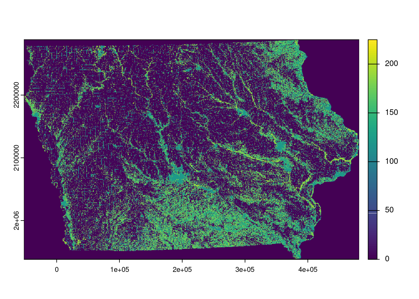
if (!require("pacman")) install.packages("pacman")
pacman::p_load(terra, tidyterra, raster, exactextractr, sf, dplyr, tidyr, data.table, prism, tictoc, tigris)
#--- set the path to the folder to which you save the downloaded PRISM data ---#
# This code sets the current working directory as the designated folder
options(prism.path = "Data")
#--- download PRISM precipitation data ---#
prism::get_prism_dailys(
type = "tmax",
date = "2018-07-01",
keepZip = FALSE
)
  |
  |                                                                      |   0%
PRISM_tmax_stable_4kmD2_20180701_bil.zip already exists. Skipping downloading.
  |
  |======================================================================| 100%
#--- the file name of the PRISM data just downloaded ---#
prism_file <- "Data/PRISM_tmax_stable_4kmD2_20180701_bil/PRISM_tmax_stable_4kmD2_20180701_bil.bil"
#--- read in the prism data ---#
prism_tmax_0701_sr <- terra::rast(prism_file)
#--- Kansas boundary (sf) ---#
KS_county_sf <-
#--- get Kansas county boundary ---
tigris::counties(state = "Kansas", cb = TRUE) %>%
#--- sp to sf ---#
sf::st_as_sf() %>%
#--- transform using the CRS of the PRISM tmax data ---#
sf::st_transform(terra::crs(prism_tmax_0701_sr))Retrieving data for the year 2022
Downloading: 16 kB
Downloading: 16 kB
Downloading: 97 kB
Downloading: 97 kB
Downloading: 160 kB
Downloading: 160 kB
Downloading: 280 kB
Downloading: 280 kB
Downloading: 410 kB
Downloading: 410 kB
Downloading: 540 kB
Downloading: 540 kB
Downloading: 670 kB
Downloading: 670 kB
Downloading: 820 kB
Downloading: 820 kB
Downloading: 830 kB
Downloading: 830 kB
Downloading: 870 kB
Downloading: 870 kB
Downloading: 880 kB
Downloading: 880 kB
Downloading: 980 kB
Downloading: 980 kB
Downloading: 1 MB
Downloading: 1 MB
Downloading: 1.1 MB
Downloading: 1.1 MB
Downloading: 1.1 MB
Downloading: 1.1 MB
Downloading: 1.1 MB
Downloading: 1.1 MB
Downloading: 1.2 MB
Downloading: 1.2 MB
Downloading: 1.2 MB
Downloading: 1.2 MB
Downloading: 1.4 MB
Downloading: 1.4 MB
Downloading: 1.6 MB
Downloading: 1.6 MB
Downloading: 1.7 MB
Downloading: 1.7 MB
Downloading: 1.7 MB
Downloading: 1.7 MB
Downloading: 1.8 MB
Downloading: 1.8 MB
Downloading: 1.9 MB
Downloading: 1.9 MB
Downloading: 2.1 MB
Downloading: 2.1 MB
Downloading: 2.3 MB
Downloading: 2.3 MB
Downloading: 2.4 MB
Downloading: 2.4 MB
Downloading: 2.5 MB
Downloading: 2.5 MB
Downloading: 2.6 MB
Downloading: 2.6 MB
Downloading: 2.8 MB
Downloading: 2.8 MB
Downloading: 2.8 MB
Downloading: 2.8 MB
Downloading: 3.1 MB
Downloading: 3.1 MB
Downloading: 3.1 MB
Downloading: 3.1 MB
Downloading: 3.3 MB
Downloading: 3.3 MB
Downloading: 3.4 MB
Downloading: 3.4 MB
Downloading: 3.6 MB
Downloading: 3.6 MB
Downloading: 3.7 MB
Downloading: 3.7 MB
Downloading: 3.8 MB
Downloading: 3.8 MB
Downloading: 3.9 MB
Downloading: 3.9 MB
Downloading: 4 MB
Downloading: 4 MB
Downloading: 4.2 MB
Downloading: 4.2 MB
Downloading: 4.3 MB
Downloading: 4.3 MB
Downloading: 4.5 MB
Downloading: 4.5 MB
Downloading: 4.5 MB
Downloading: 4.5 MB
Downloading: 4.6 MB
Downloading: 4.6 MB
Downloading: 4.6 MB
Downloading: 4.6 MB
Downloading: 4.9 MB
Downloading: 4.9 MB
Downloading: 5.1 MB
Downloading: 5.1 MB
Downloading: 5.3 MB
Downloading: 5.3 MB
Downloading: 5.5 MB
Downloading: 5.5 MB
Downloading: 5.6 MB
Downloading: 5.6 MB
Downloading: 5.7 MB
Downloading: 5.7 MB
Downloading: 5.8 MB
Downloading: 5.8 MB
Downloading: 5.9 MB
Downloading: 5.9 MB
Downloading: 5.9 MB
Downloading: 5.9 MB
Downloading: 6 MB
Downloading: 6 MB
Downloading: 6.1 MB
Downloading: 6.1 MB
Downloading: 6.2 MB
Downloading: 6.2 MB
Downloading: 6.3 MB
Downloading: 6.3 MB
Downloading: 6.4 MB
Downloading: 6.4 MB
Downloading: 6.5 MB
Downloading: 6.5 MB
Downloading: 6.5 MB
Downloading: 6.5 MB
Downloading: 6.7 MB
Downloading: 6.7 MB
Downloading: 6.9 MB
Downloading: 6.9 MB
Downloading: 7.1 MB
Downloading: 7.1 MB
Downloading: 7.3 MB
Downloading: 7.3 MB
Downloading: 7.4 MB
Downloading: 7.4 MB
Downloading: 7.6 MB
Downloading: 7.6 MB
Downloading: 7.6 MB
Downloading: 7.6 MB
Downloading: 7.7 MB
Downloading: 7.7 MB
Downloading: 7.8 MB
Downloading: 7.8 MB
Downloading: 8 MB
Downloading: 8 MB
Downloading: 8 MB
Downloading: 8 MB
Downloading: 8.2 MB
Downloading: 8.2 MB
Downloading: 8.2 MB
Downloading: 8.2 MB
Downloading: 8.3 MB
Downloading: 8.3 MB
Downloading: 8.4 MB
Downloading: 8.4 MB
Downloading: 8.5 MB
Downloading: 8.5 MB
Downloading: 8.6 MB
Downloading: 8.6 MB
Downloading: 8.8 MB
Downloading: 8.8 MB
Downloading: 9 MB
Downloading: 9 MB
Downloading: 9.2 MB
Downloading: 9.2 MB
Downloading: 9.3 MB
Downloading: 9.3 MB
Downloading: 9.4 MB
Downloading: 9.4 MB
Downloading: 9.5 MB
Downloading: 9.5 MB
Downloading: 9.7 MB
Downloading: 9.7 MB
Downloading: 9.9 MB
Downloading: 9.9 MB
Downloading: 9.9 MB
Downloading: 9.9 MB
Downloading: 10 MB
Downloading: 10 MB
Downloading: 10 MB
Downloading: 10 MB
Downloading: 10 MB
Downloading: 10 MB
Downloading: 11 MB
Downloading: 11 MB
Downloading: 11 MB
Downloading: 11 MB
Downloading: 11 MB
Downloading: 11 MB
Downloading: 11 MB
Downloading: 11 MB
Downloading: 12 MB
Downloading: 12 MB
Downloading: 12 MB
Downloading: 12 MB
# terra::(SpatRaster, sf)
prism_tmax_0701_KS_sr <-
terra::crop(
prism_tmax_0701_sr,
KS_county_sf
)
library(tidyverse)── Attaching core tidyverse packages ──────────────────────── tidyverse 2.0.0 ──
✔ forcats 1.0.0 ✔ readr 2.1.5
✔ ggplot2 3.5.1 ✔ stringr 1.5.1
✔ purrr 1.0.4 ✔ tibble 3.2.1
── Conflicts ────────────────────────────────────────── tidyverse_conflicts() ──
✖ data.table::between() masks dplyr::between()
✖ tidyr::extract() masks raster::extract(), terra::extract()
✖ tidyterra::filter() masks dplyr::filter(), stats::filter()
✖ data.table::first() masks dplyr::first()
✖ data.table::hour() masks lubridate::hour()
✖ data.table::isoweek() masks lubridate::isoweek()
✖ dplyr::lag() masks stats::lag()
✖ data.table::last() masks dplyr::last()
✖ data.table::mday() masks lubridate::mday()
✖ data.table::minute() masks lubridate::minute()
✖ data.table::month() masks lubridate::month()
✖ data.table::quarter() masks lubridate::quarter()
✖ data.table::second() masks lubridate::second()
✖ tidyterra::select() masks dplyr::select(), raster::select()
✖ purrr::transpose() masks data.table::transpose()
✖ data.table::wday() masks lubridate::wday()
✖ data.table::week() masks lubridate::week()
✖ data.table::yday() masks lubridate::yday()
✖ data.table::year() masks lubridate::year()
ℹ Use the conflicted package (<http://conflicted.r-lib.org/>) to force all conflicts to become errorsggplot() +
geom_spatraster(data = prism_tmax_0701_KS_sr) +
geom_sf(data = KS_county_sf, fill = NA, color = "blue") +
scale_fill_whitebox_c(
name = "tmax",
palette = "muted",
labels = scales::label_number(suffix = "o"),
n.breaks = 12,
guide = guide_legend(reverse = TRUE)
) +
theme_void()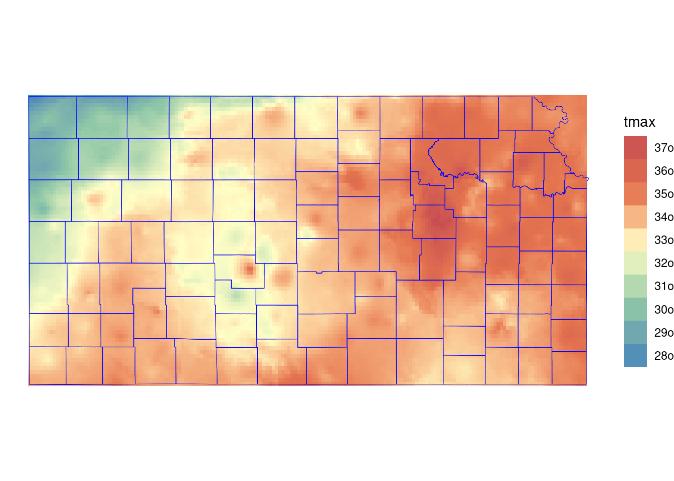
#--- download PRISM precipitation data ---#
prism::get_prism_dailys(
  type = "tmax",
  date = "2018-07-02",
  keepZip = FALSE
)
  |
  |                                                                      |   0%
PRISM_tmax_stable_4kmD2_20180702_bil.zip already exists. Skipping downloading.
  |
  |======================================================================| 100%
#--- the file name of the PRISM data just downloaded ---#
prism_file <- "Data/PRISM_tmax_stable_4kmD2_20180702_bil/PRISM_tmax_stable_4kmD2_20180702_bil.bil"
#--- read in the prism data and crop it to Kansas state border ---#
prism_tmax_0702_KS_sr <-
terra::rast(prism_file) %>%
terra::crop(KS_county_sf)
#--- read in the KS points data ---#
(
KS_wells <- readRDS("Data/Chap_5_wells_KS.rds")
)Simple feature collection with 37647 features and 1 field
Geometry type: POINT
Dimension: XY
Bounding box: xmin: -102.0495 ymin: 36.99552 xmax: -94.62089 ymax: 40.00199
Geodetic CRS: NAD83
First 10 features:
well_id geometry
1 1 POINT (-100.4423 37.52046)
2 3 POINT (-100.7118 39.91526)
3 5 POINT (-99.15168 38.48849)
4 7 POINT (-101.8995 38.78077)
5 8 POINT (-100.7122 38.0731)
6 9 POINT (-97.70265 39.04055)
7 11 POINT (-101.7114 39.55035)
8 12 POINT (-95.97031 39.16121)
9 15 POINT (-98.30759 38.26787)
10 17 POINT (-100.2785 37.71539)ggplot() +
geom_sf(data = KS_county_sf, fill = NA) +
geom_sf(data = KS_wells, size = 0.05) +
theme_void()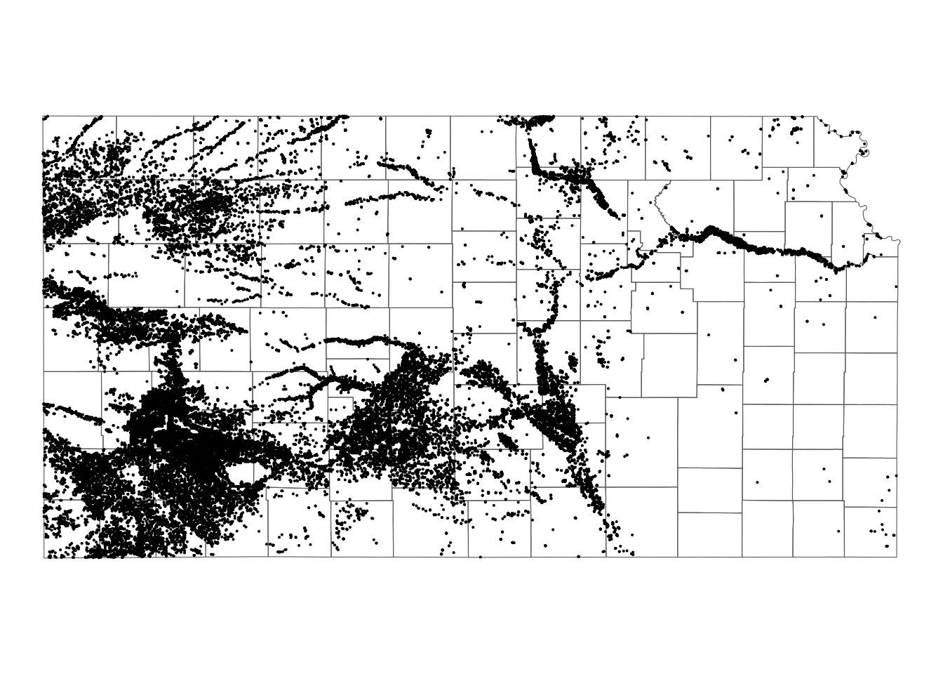
# terra:extract(raster, points)

tmax_from_prism <- terra::extract(prism_tmax_0701_KS_sr, KS_wells)

head(tmax_from_prism)
ID PRISM_tmax_stable_4kmD2_20180701_bil
1 1 34.241
2 2 29.288
3 3 32.585
4 4 30.104
5 5 34.232
6 6 35.168KS_wells$tmax_07_01 <- tmax_from_prism[,-1]#--- create a multi-layer SpatRaster ---#
prism_tmax_stack <- c(prism_tmax_0701_KS_sr, prism_tmax_0702_KS_sr)
#--- extract tmax values ---#
tmax_from_prism_stack <- terra::extract(prism_tmax_stack, KS_wells)
#--- take a look ---#
head(tmax_from_prism_stack) ID PRISM_tmax_stable_4kmD2_20180701_bil PRISM_tmax_stable_4kmD2_20180702_bil
1 1 34.241 30.544
2 2 29.288 29.569
3 3 32.585 29.866
4 4 30.104 29.819
5 5 34.232 30.481
6 6 35.168 30.640tmax_by_county <- terra::extract(prism_tmax_0701_KS_sr, KS_county_sf)
class(tmax_by_county)[1] "data.frame"head(tmax_by_county) ID PRISM_tmax_stable_4kmD2_20180701_bil
1 1 34.181
2 1 34.180
3 1 34.210
4 1 34.190
5 1 34.292
6 1 34.258#--- get mean tmax ---#
mean_tmax <-
tmax_by_county %>%
group_by(ID) %>%
summarize(tmax = mean(PRISM_tmax_stable_4kmD2_20180701_bil))
(
KS_county_sf <-
#--- back to sf ---#
KS_county_sf %>%
#--- define ID ---#
mutate(ID := seq_len(nrow(.))) %>%
#--- merge by ID ---#
left_join(., mean_tmax, by = "ID")
)Simple feature collection with 105 features and 14 fields
Geometry type: MULTIPOLYGON
Dimension: XY
Bounding box: xmin: -102.0517 ymin: 36.99302 xmax: -94.58841 ymax: 40.00316
Geodetic CRS: NAD83
First 10 features:
STATEFP COUNTYFP COUNTYNS AFFGEOID GEOID NAME
1 20 175 00485050 0500000US20175 20175 Seward
2 20 027 00484983 0500000US20027 20027 Clay
3 20 171 00485048 0500000US20171 20171 Scott
4 20 047 00484993 0500000US20047 20047 Edwards
5 20 147 00485037 0500000US20147 20147 Phillips
6 20 149 00485038 0500000US20149 20149 Pottawatomie
7 20 055 00485326 0500000US20055 20055 Finney
8 20 167 00485046 0500000US20167 20167 Russell
9 20 135 00485031 0500000US20135 20135 Ness
10 20 093 00485011 0500000US20093 20093 Kearny
NAMELSAD STUSPS STATE_NAME LSAD ALAND AWATER ID tmax
1 Seward County KS Kansas 06 1656693304 1961444 1 34.47948
2 Clay County KS Kansas 06 1671314413 26701337 2 34.51894
3 Scott County KS Kansas 06 1858536838 306079 3 33.56413
4 Edwards County KS Kansas 06 1610699245 206413 4 32.26368
5 Phillips County KS Kansas 06 2294395636 22493383 5 32.57836
6 Pottawatomie County KS Kansas 06 2177493041 54149843 6 35.67524
7 Finney County KS Kansas 06 3372157854 1716371 7 33.96920
8 Russell County KS Kansas 06 2295402858 34126776 8 33.37254
9 Ness County KS Kansas 06 2783562234 667491 9 32.86275
10 Kearny County KS Kansas 06 2254696661 1133601 10 33.40829
geometry
1 MULTIPOLYGON (((-101.0681 3...
2 MULTIPOLYGON (((-97.3707 39...
3 MULTIPOLYGON (((-101.1284 3...
4 MULTIPOLYGON (((-99.56988 3...
5 MULTIPOLYGON (((-99.62821 3...
6 MULTIPOLYGON (((-96.72774 3...
7 MULTIPOLYGON (((-101.103 37...
8 MULTIPOLYGON (((-99.04234 3...
9 MULTIPOLYGON (((-100.2477 3...
10 MULTIPOLYGON (((-101.5419 3...tmax_by_county <-
terra::extract(
prism_tmax_0701_KS_sr,
KS_county_sf,
fun = mean
)
head(tmax_by_county) ID PRISM_tmax_stable_4kmD2_20180701_bil
1 1 34.47948
2 2 34.51894
3 3 33.56413
4 4 32.26368
5 5 32.57836
6 6 35.67524# exactextractr::exact_extract(raster, polygons sf, include_cols = list of vars)
tmax_by_county <-
exactextractr::exact_extract(
prism_tmax_0701_KS_sr,
KS_county_sf,
include_cols = "COUNTYFP",
progress = FALSE
)
tmax_by_county[1:2] %>% lapply(function(x) head(x))[[1]]
COUNTYFP value coverage_fraction
1 175 34.222 0.1074141
2 175 34.181 0.8066747
3 175 34.180 0.8066615
4 175 34.210 0.8066448
5 175 34.190 0.8061629
6 175 34.292 0.8054324
[[2]]
COUNTYFP value coverage_fraction
1 027 33.847 0.03732148
2 027 33.897 0.10592906
3 027 34.010 0.10249268
4 027 34.186 0.10018899
5 027 34.293 0.10074520
6 027 34.220 0.09701102tmax_combined <- tmax_by_county %>%
dplyr::bind_rows() %>%
tibble::as_tibble()Stars packageif (!require("pacman")) install.packages("pacman")
pacman::p_load(
stars, # spatiotemporal data handling
sf, # vector data handling
tidyverse, # data wrangling
cubelyr, # handle raster data
mapview, # make maps
exactextractr, # fast raster data extraction
lubridate, # handle dates
prism # download PRISM data
)