if (!require("pacman")) install.packages("pacman")
pacman::p_load(
  sf, # vector data operations
  tidyverse, # data wrangling
  data.table, # data wrangling
  tmap, # make maps
  mapview, # create an interactive map
  patchwork, # arranging maps
  rmapshaper
)Geospatial with R
Handling vector data with sf
This is my practice sections following R as GIS for Economists.
Basics
Load the packages:
#--- a dataset that comes with the sf package ---#
nc <- sf::st_read(system.file("shape/nc.shp", package = "sf"))
Reading layer `nc' from data source
`/home/himakun/R/x86_64-pc-linux-gnu-library/4.4/sf/shape/nc.shp'
using driver `ESRI Shapefile'
Simple feature collection with 100 features and 14 fields
Geometry type: MULTIPOLYGON
Dimension: XY
Bounding box: xmin: -84.32385 ymin: 33.88199 xmax: -75.45698 ymax: 36.58965
Geodetic CRS: NAD27ggplot() +
geom_sf(data = nc) +
theme_void()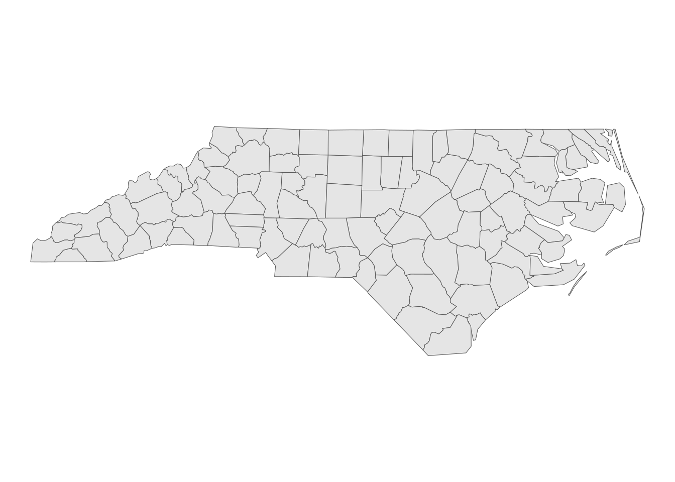
head(nc)Simple feature collection with 6 features and 14 fields
Geometry type: MULTIPOLYGON
Dimension: XY
Bounding box: xmin: -81.74107 ymin: 36.07282 xmax: -75.77316 ymax: 36.58965
Geodetic CRS: NAD27
AREA PERIMETER CNTY_ CNTY_ID NAME FIPS FIPSNO CRESS_ID BIR74 SID74
1 0.114 1.442 1825 1825 Ashe 37009 37009 5 1091 1
2 0.061 1.231 1827 1827 Alleghany 37005 37005 3 487 0
3 0.143 1.630 1828 1828 Surry 37171 37171 86 3188 5
4 0.070 2.968 1831 1831 Currituck 37053 37053 27 508 1
5 0.153 2.206 1832 1832 Northampton 37131 37131 66 1421 9
6 0.097 1.670 1833 1833 Hertford 37091 37091 46 1452 7
NWBIR74 BIR79 SID79 NWBIR79 geometry
1 10 1364 0 19 MULTIPOLYGON (((-81.47276 3...
2 10 542 3 12 MULTIPOLYGON (((-81.23989 3...
3 208 3616 6 260 MULTIPOLYGON (((-80.45634 3...
4 123 830 2 145 MULTIPOLYGON (((-76.00897 3...
5 1066 1606 3 1197 MULTIPOLYGON (((-77.21767 3...
6 954 1838 5 1237 MULTIPOLYGON (((-76.74506 3...sfg: LINESTRING
#--- collection of points in a matrix form ---#
s1 <- rbind(c(2, 3), c(3, 4), c(3, 5), c(1, 5))

#--- see what s1 looks like ---#
s1
[,1] [,2]
[1,] 2 3
[2,] 3 4
[3,] 3 5
[4,] 1 5#--- create a "LINESTRING" ---#
a_linestring <- sf::st_linestring(s1)
#--- check the class ---#
class(a_linestring)[1] "XY" "LINESTRING" "sfg" sfg: POLYGON
#--- a hole within p1 ---#
p1 <- rbind(c(0, 0), c(3, 0), c(3, 2), c(2, 5), c(1, 3), c(0, 0))
p2 <- rbind(c(1, 1), c(1, 2), c(2, 2), c(1, 1))

#--- create a polygon with hole ---#
a_plygon_with_a_hole <- sf::st_polygon(list(p1, p2))

plot(a_plygon_with_a_hole)
Creating sfc object or sf object:
#--- create an sfc ---#
sfc_ex <- sf::st_sfc(list(a_linestring, a_plygon_with_a_hole))

#--- create a data.frame ---#
df_ex <- data.frame(name = c("A", "B"))

#--- add the sfc as a column ---#
df_ex$geometry <- sfc_ex

#--- take a look ---#
df_ex
name geometry
1 A LINESTRING (2 3, 3 4, 3 5, ...
2 B POLYGON ((0 0, 3 0, 3 2, 2 ...#--- let R recognize the data frame as sf ---#
sf_ex <- sf::st_as_sf(df_ex)
#--- see what it looks like ---#
sf_exSimple feature collection with 2 features and 1 field
Geometry type: GEOMETRY
Dimension: XY
Bounding box: xmin: 0 ymin: 0 xmax: 3 ymax: 5
CRS: NA
  name                       geometry
1    A LINESTRING (2 3, 3 4, 3 5, ...
2 B POLYGON ((0 0, 3 0, 3 2, 2 ...Read shapefile:
#--- read a NE county boundary shapefile ---#
nc_loaded <- sf::st_read("Data/nc.shp")
Reading layer `nc' from data source
`/home/himakun/Documents/tools/computing/Data/nc.shp' using driver `ESRI Shapefile'
Simple feature collection with 100 features and 1 field
Geometry type: MULTIPOLYGON
Dimension: XY
Bounding box: xmin: -84.32385 ymin: 33.88199 xmax: -75.45698 ymax: 36.58965
Geodetic CRS: NAD27Projection with different CRS:
sf::st_crs(nc)Coordinate Reference System:
User input: NAD27
wkt:
GEOGCRS["NAD27",
DATUM["North American Datum 1927",
ELLIPSOID["Clarke 1866",6378206.4,294.978698213898,
LENGTHUNIT["metre",1]]],
PRIMEM["Greenwich",0,
ANGLEUNIT["degree",0.0174532925199433]],
CS[ellipsoidal,2],
AXIS["latitude",north,
ORDER[1],
ANGLEUNIT["degree",0.0174532925199433]],
AXIS["longitude",east,
ORDER[2],
ANGLEUNIT["degree",0.0174532925199433]],
ID["EPSG",4267]]Change the CRS projection:
#--- transform ---#
nc_wgs84 <- sf::st_transform(nc, 4326)

#--- check if the transformation was successful ---#
sf::st_crs(nc_wgs84)
Coordinate Reference System:
User input: EPSG:4326
wkt:
GEOGCRS["WGS 84",
ENSEMBLE["World Geodetic System 1984 ensemble",
MEMBER["World Geodetic System 1984 (Transit)"],
MEMBER["World Geodetic System 1984 (G730)"],
MEMBER["World Geodetic System 1984 (G873)"],
MEMBER["World Geodetic System 1984 (G1150)"],
MEMBER["World Geodetic System 1984 (G1674)"],
MEMBER["World Geodetic System 1984 (G1762)"],
MEMBER["World Geodetic System 1984 (G2139)"],
ELLIPSOID["WGS 84",6378137,298.257223563,
LENGTHUNIT["metre",1]],
ENSEMBLEACCURACY[2.0]],
PRIMEM["Greenwich",0,
ANGLEUNIT["degree",0.0174532925199433]],
CS[ellipsoidal,2],
AXIS["geodetic latitude (Lat)",north,
ORDER[1],
ANGLEUNIT["degree",0.0174532925199433]],
AXIS["geodetic longitude (Lon)",east,
ORDER[2],
ANGLEUNIT["degree",0.0174532925199433]],
USAGE[
SCOPE["Horizontal component of 3D system."],
AREA["World."],
BBOX[-90,-180,90,180]],
ID["EPSG",4326]]#--- transform ---#
nc_utm17N <- sf::st_transform(nc_wgs84, 26917)
#--- check if the transformation was successful ---#
sf::st_crs(nc_utm17N)Coordinate Reference System:
User input: EPSG:26917
wkt:
PROJCRS["NAD83 / UTM zone 17N",
BASEGEOGCRS["NAD83",
DATUM["North American Datum 1983",
ELLIPSOID["GRS 1980",6378137,298.257222101,
LENGTHUNIT["metre",1]]],
PRIMEM["Greenwich",0,
ANGLEUNIT["degree",0.0174532925199433]],
ID["EPSG",4269]],
CONVERSION["UTM zone 17N",
METHOD["Transverse Mercator",
ID["EPSG",9807]],
PARAMETER["Latitude of natural origin",0,
ANGLEUNIT["degree",0.0174532925199433],
ID["EPSG",8801]],
PARAMETER["Longitude of natural origin",-81,
ANGLEUNIT["degree",0.0174532925199433],
ID["EPSG",8802]],
PARAMETER["Scale factor at natural origin",0.9996,
SCALEUNIT["unity",1],
ID["EPSG",8805]],
PARAMETER["False easting",500000,
LENGTHUNIT["metre",1],
ID["EPSG",8806]],
PARAMETER["False northing",0,
LENGTHUNIT["metre",1],
ID["EPSG",8807]]],
CS[Cartesian,2],
AXIS["(E)",east,
ORDER[1],
LENGTHUNIT["metre",1]],
AXIS["(N)",north,
ORDER[2],
LENGTHUNIT["metre",1]],
USAGE[
SCOPE["Engineering survey, topographic mapping."],
AREA["North America - between 84°W and 78°W - onshore and offshore. Canada - Nunavut; Ontario; Quebec. United States (USA) - Florida; Georgia; Kentucky; Maryland; Michigan; New York; North Carolina; Ohio; Pennsylvania; South Carolina; Tennessee; Virginia; West Virginia."],
BBOX[23.81,-84,84,-78]],
ID["EPSG",26917]]#--- transform ---#
nc_utm17N_2 <- sf::st_transform(nc_wgs84, sf::st_crs(nc_utm17N))
#--- check if the transformation was successful ---#
sf::st_crs(nc_utm17N_2)Coordinate Reference System:
User input: EPSG:26917
wkt:
PROJCRS["NAD83 / UTM zone 17N",
BASEGEOGCRS["NAD83",
DATUM["North American Datum 1983",
ELLIPSOID["GRS 1980",6378137,298.257222101,
LENGTHUNIT["metre",1]]],
PRIMEM["Greenwich",0,
ANGLEUNIT["degree",0.0174532925199433]],
ID["EPSG",4269]],
CONVERSION["UTM zone 17N",
METHOD["Transverse Mercator",
ID["EPSG",9807]],
PARAMETER["Latitude of natural origin",0,
ANGLEUNIT["degree",0.0174532925199433],
ID["EPSG",8801]],
PARAMETER["Longitude of natural origin",-81,
ANGLEUNIT["degree",0.0174532925199433],
ID["EPSG",8802]],
PARAMETER["Scale factor at natural origin",0.9996,
SCALEUNIT["unity",1],
ID["EPSG",8805]],
PARAMETER["False easting",500000,
LENGTHUNIT["metre",1],
ID["EPSG",8806]],
PARAMETER["False northing",0,
LENGTHUNIT["metre",1],
ID["EPSG",8807]]],
CS[Cartesian,2],
AXIS["(E)",east,
ORDER[1],
LENGTHUNIT["metre",1]],
AXIS["(N)",north,
ORDER[2],
LENGTHUNIT["metre",1]],
USAGE[
SCOPE["Engineering survey, topographic mapping."],
AREA["North America - between 84°W and 78°W - onshore and offshore. Canada - Nunavut; Ontario; Quebec. United States (USA) - Florida; Georgia; Kentucky; Maryland; Michigan; New York; North Carolina; Ohio; Pennsylvania; South Carolina; Tennessee; Virginia; West Virginia."],
BBOX[23.81,-84,84,-78]],
ID["EPSG",26917]]Turning dataframe into sf object
#--- read irrigation well registration data ---#
(
  wells <- readRDS("Data/well_registration.rds")
)
Key: <wellid>
wellid ownerid nrdname acres regdate section longdd
<int> <int> <char> <num> <char> <int> <num>
1: 2 106106 Central Platte 160 12/30/55 3 -99.58401
2: 3 14133 South Platte 46 4/29/31 8 -102.62495
3: 4 14133 South Platte 46 4/29/31 8 -102.62495
4: 5 14133 South Platte 46 4/29/31 8 -102.62495
5: 6 15837 Central Platte 160 8/29/32 20 -99.62580
---
105818: 244568 135045 Upper Big Blue NA 8/26/16 30 -97.58872
105819: 244569 105428 Little Blue NA 8/26/16 24 -97.60752
105820: 244570 135045 Upper Big Blue NA 8/26/16 30 -97.58294
105821: 244571 135045 Upper Big Blue NA 8/26/16 25 -97.59775
105822: 244572 105428 Little Blue NA 8/26/16 15 -97.64086
latdd
<num>
1: 40.69825
2: 41.11699
3: 41.11699
4: 41.11699
5: 40.73268
---
105818: 40.89017
105819: 40.13257
105820: 40.88722
105821: 40.89639
105822: 40.13380#--- recognize it as an sf ---#
wells_sf <- sf::st_as_sf(wells, coords = c("longdd", "latdd")) %>%
st_set_crs(4269)
#--- take a look at the data ---#
head(wells_sf[, 1:5])Simple feature collection with 6 features and 5 fields
Geometry type: POINT
Dimension: XY
Bounding box: xmin: -102.6249 ymin: 40.69824 xmax: -99.58401 ymax: 41.11699
Geodetic CRS: NAD83
wellid ownerid nrdname acres regdate geometry
1 2 106106 Central Platte 160 12/30/55 POINT (-99.58401 40.69825)
2 3 14133 South Platte 46 4/29/31 POINT (-102.6249 41.11699)
3 4 14133 South Platte 46 4/29/31 POINT (-102.6249 41.11699)
4 5 14133 South Platte 46 4/29/31 POINT (-102.6249 41.11699)
5 6 15837 Central Platte 160 8/29/32 POINT (-99.6258 40.73268)
6 7 90248 Central Platte 120 2/15/35 POINT (-99.64524 40.73164)Conversion to and from sp objects
#--- conversion ---#
wells_sp <- as(wells_sf, "Spatial")

#--- check the class ---#
class(wells_sp)
[1] "SpatialPointsDataFrame"
attr(,"package")
[1] "sp"#--- revert back to sf ---#
wells_sf <- sf::st_as_sf(wells_sp)
#--- check the class ---#
class(wells_sf)[1] "sf" "data.frame"Reverting sf object back into dataframe
#--- remove geometry ---#
wells_no_longer_sf <- sf::st_drop_geometry(wells_sf)

#--- take a look ---#
head(wells_no_longer_sf)
wellid ownerid nrdname acres regdate section
1 2 106106 Central Platte 160 12/30/55 3
2 3 14133 South Platte 46 4/29/31 8
3 4 14133 South Platte 46 4/29/31 8
4 5 14133 South Platte 46 4/29/31 8
5 6 15837 Central Platte 160 8/29/32 20
6 7 90248 Central Platte 120 2/15/35 19#--- read wells location data ---#
urnrd_wells_sf <-
readRDS("Data/urnrd_wells.rds") %>%
#--- project to UTM 14N WGS 84 ---#
sf::st_transform(32614)
#--- create a one-mile buffer around the wells ---#
wells_buffer <- sf::st_buffer(urnrd_wells_sf, dist = 1600)
head(wells_buffer)Simple feature collection with 6 features and 6 fields
Geometry type: POLYGON
Dimension: XY
Bounding box: xmin: 251786.6 ymin: 4483187 xmax: 301596 ymax: 4499464
Projected CRS: WGS 84 / UTM zone 14N
wellid ownerid nrdname acres regdate section
1 79 98705 Upper Republican 400 12/9/40 5
2 109 115260 Upper Republican 80 3/11/41 20
3 161 115260 Upper Republican 50 3/8/43 17
4 162 41350 Upper Republican 140 3/23/43 28
5 164 105393 Upper Republican 90 7/6/43 12
6 166 51341 Upper Republican 110 8/31/43 18
geometry
1 POLYGON ((277371.9 4497864,...
2 POLYGON ((256979.6 4484787,...
3 POLYGON ((256993.1 4485173,...
4 POLYGON ((258354.5 4492808,...
5 POLYGON ((301596 4485998, 3...
6 POLYGON ((254986.6 4485670,...ggplot() +
geom_sf(data = urnrd_wells_sf, size = 0.6, color = "red") +
geom_sf(data = wells_buffer, fill = NA) +
theme_void()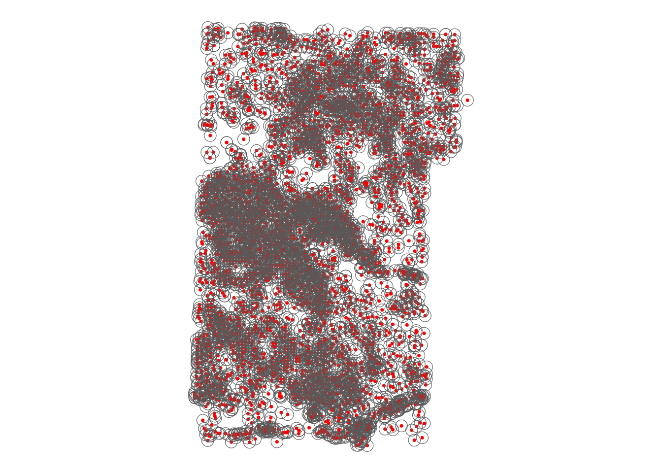
NE_counties <-
  readRDS("Data/NE_county_borders.rds") %>%
  dplyr::filter(NAME %in% c("Perkins", "Dundy", "Chase")) %>%
  sf::st_transform(32614)

#--- generate area by polygon ---#
(
  NE_counties <- dplyr::mutate(NE_counties, area = st_area(NE_counties))
)
Simple feature collection with 3 features and 10 fields
Geometry type: MULTIPOLYGON
Dimension: XY
Bounding box: xmin: 239494.1 ymin: 4430632 xmax: 310778.1 ymax: 4543676
Projected CRS: WGS 84 / UTM zone 14N
STATEFP COUNTYFP COUNTYNS AFFGEOID GEOID NAME LSAD ALAND
1 31 135 00835889 0500000US31135 31135 Perkins 06 2287828025
2 31 029 00835836 0500000US31029 31029 Chase 06 2316533447
3 31 057 00835850 0500000US31057 31057 Dundy 06 2381956151
AWATER geometry area
1 2840176 MULTIPOLYGON (((243340.2 45... 2302174854 [m^2]
2 7978172 MULTIPOLYGON (((241201.4 44... 2316908196 [m^2]
3 3046331 MULTIPOLYGON (((240811.3 44... 2389890530 [m^2]#--- create centroids ---#
(
NE_centroids <- sf::st_centroid(NE_counties)
)Warning: st_centroid assumes attributes are constant over geometriesSimple feature collection with 3 features and 10 fields
Geometry type: POINT
Dimension: XY
Bounding box: xmin: 271156.7 ymin: 4450826 xmax: 276594.1 ymax: 4525635
Projected CRS: WGS 84 / UTM zone 14N
STATEFP COUNTYFP COUNTYNS AFFGEOID GEOID NAME LSAD ALAND
1 31 135 00835889 0500000US31135 31135 Perkins 06 2287828025
2 31 029 00835836 0500000US31029 31029 Chase 06 2316533447
3 31 057 00835850 0500000US31057 31057 Dundy 06 2381956151
AWATER geometry area
1 2840176 POINT (276594.1 4525635) 2302174854 [m^2]
2 7978172 POINT (271469.9 4489429) 2316908196 [m^2]
3 3046331 POINT (271156.7 4450826) 2389890530 [m^2]ggplot() +
geom_sf(data = NE_counties) +
geom_sf_text(data = NE_centroids, aes(label = NAME)) +
theme_void()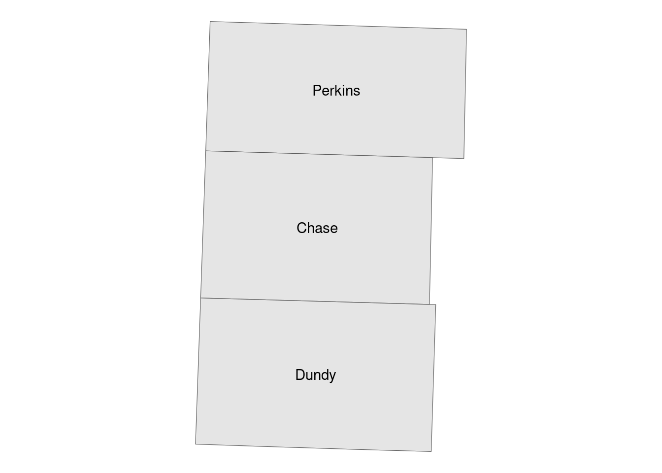
IL_counties <- sf::st_read("Data/IL_county_detailed.geojson")Reading layer `IL_county_detailed' from data source
`/home/himakun/Documents/tools/computing/Data/IL_county_detailed.geojson'
using driver `GeoJSON'
Simple feature collection with 102 features and 61 fields
Geometry type: MULTIPOLYGON
Dimension: XY
Bounding box: xmin: -91.51309 ymin: 36.9703 xmax: -87.4952 ymax: 42.50849
Geodetic CRS: WGS 84IL_counties_mssimplified <- rmapshaper::ms_simplify(IL_counties, keep = 0.01)
Cook <- filter(IL_counties, NAME == "Cook County")
Cook_simplify <- sf::st_simplify(Cook, dTolerance = 1000)
ggplot() +
geom_sf(data = Cook_simplify) +
theme_void()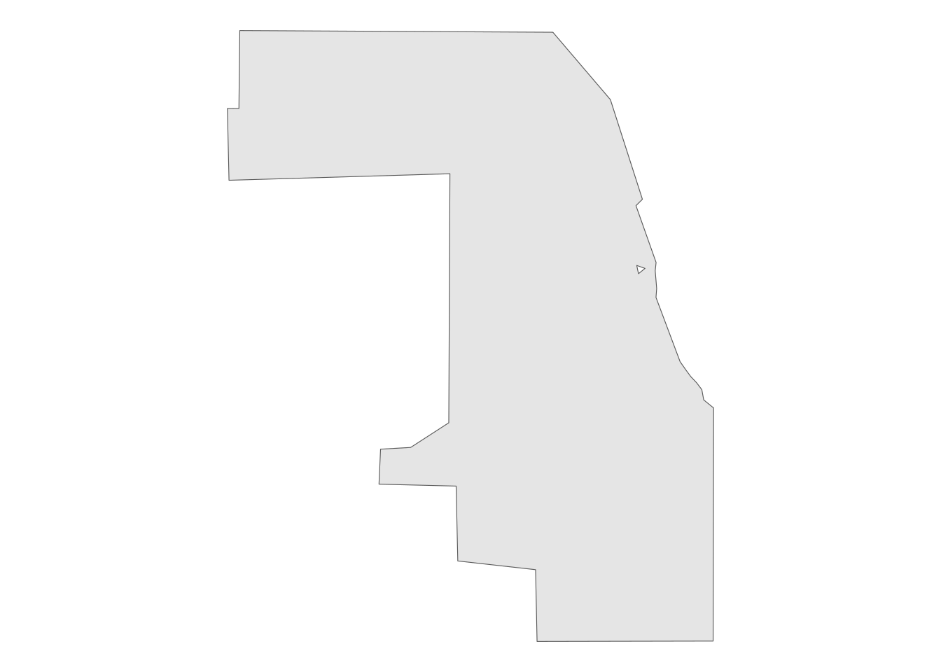
Spatial Interactions of Vector Data: Subsetting and Joining
#--- create points ---#
point_1 <- sf::st_point(c(2, 2))
point_2 <- sf::st_point(c(1, 1))
point_3 <- sf::st_point(c(1, 3))

#--- combine the points to make a single  sf of points ---#
(
points <-
  list(point_1, point_2, point_3) %>%
  sf::st_sfc() %>%
  sf::st_as_sf() %>%
  dplyr::mutate(point_name = c("point 1", "point 2", "point 3"))
)
Simple feature collection with 3 features and 1 field
Geometry type: POINT
Dimension: XY
Bounding box: xmin: 1 ymin: 1 xmax: 2 ymax: 3
CRS: NA
x point_name
1 POINT (2 2) point 1
2 POINT (1 1) point 2
3 POINT (1 3) point 3#--- create points ---#
line_1 <- sf::st_linestring(rbind(c(0, 0), c(2.5, 0.5)))
line_2 <- sf::st_linestring(rbind(c(1.5, 0.5), c(2.5, 2)))
#--- combine the points to make a single sf of points ---#
(
lines <-
list(line_1, line_2) %>%
sf::st_sfc() %>%
sf::st_as_sf() %>%
dplyr::mutate(line_name = c("line 1", "line 2"))
)Simple feature collection with 2 features and 1 field
Geometry type: LINESTRING
Dimension: XY
Bounding box: xmin: 0 ymin: 0 xmax: 2.5 ymax: 2
CRS: NA
x line_name
1 LINESTRING (0 0, 2.5 0.5) line 1
2 LINESTRING (1.5 0.5, 2.5 2) line 2#--- create polygons ---#
polygon_1 <- sf::st_polygon(list(
rbind(c(0, 0), c(2, 0), c(2, 2), c(0, 2), c(0, 0))
))
polygon_2 <- sf::st_polygon(list(
rbind(c(0.5, 1.5), c(0.5, 3.5), c(2.5, 3.5), c(2.5, 1.5), c(0.5, 1.5))
))
polygon_3 <- sf::st_polygon(list(
rbind(c(0.5, 2.5), c(0.5, 3.2), c(2.3, 3.2), c(2, 2), c(0.5, 2.5))
))
#--- combine the polygons to make an sf of polygons ---#
(
polygons <-
list(polygon_1, polygon_2, polygon_3) %>%
sf::st_sfc() %>%
sf::st_as_sf() %>%
dplyr::mutate(polygon_name = c("polygon 1", "polygon 2", "polygon 3"))
)Simple feature collection with 3 features and 1 field
Geometry type: POLYGON
Dimension: XY
Bounding box: xmin: 0 ymin: 0 xmax: 2.5 ymax: 3.5
CRS: NA
x polygon_name
1 POLYGON ((0 0, 2 0, 2 2, 0 ... polygon 1
2 POLYGON ((0.5 1.5, 0.5 3.5,... polygon 2
3 POLYGON ((0.5 2.5, 0.5 3.2,... polygon 3ggplot() +
geom_sf(data = polygons, aes(fill = polygon_name), alpha = 0.3) +
scale_fill_discrete(name = "Polygons") +
geom_sf(data = lines, aes(color = line_name)) +
scale_color_discrete(name = "Lines") +
geom_sf(data = points, aes(shape = point_name), size = 4) +
scale_shape_discrete(name = "Points") 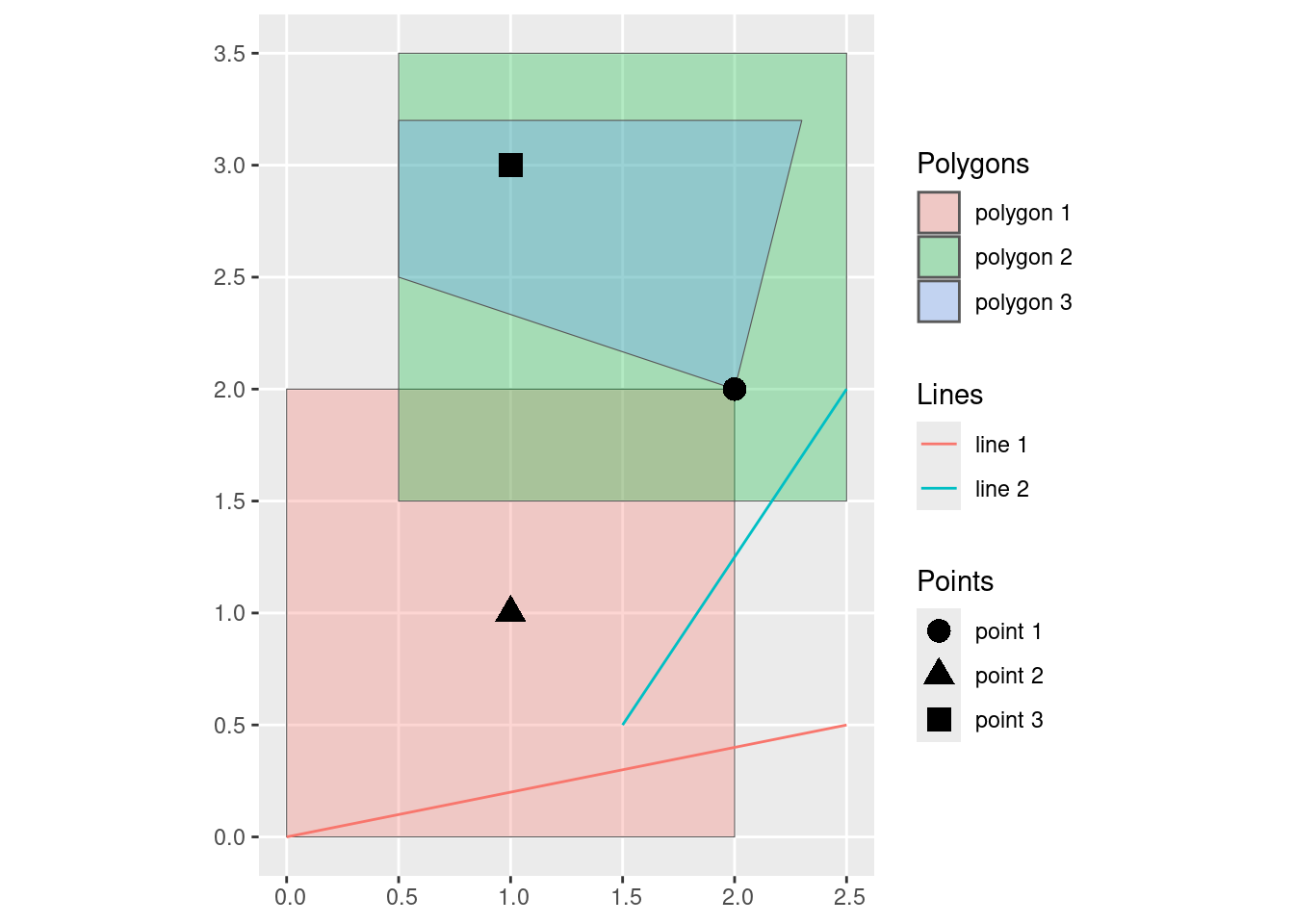
sf::st_intersects(points, polygons)Sparse geometry binary predicate list of length 3, where the predicate
was `intersects'
1: 1, 2, 3
2: 1
3: 2, 3set.seed(38424738)
points_set_1 <-
lapply(1:5, function(x) sf::st_point(runif(2))) %>%
sf::st_sfc() %>% sf::st_as_sf() %>%
dplyr::mutate(id = 1:nrow(.))
points_set_2 <-
lapply(1:5, function(x) sf::st_point(runif(2))) %>%
sf::st_sfc() %>% sf::st_as_sf() %>%
dplyr::mutate(id = 1:nrow(.))sf::st_is_within_distance(points_set_1, points_set_2, dist = 0.2)Sparse geometry binary predicate list of length 5, where the predicate
was `is_within_distance'
1: 1
2: (empty)
3: (empty)
4: (empty)
5: 3#--- Kansas county borders ---#
KS_counties <-
readRDS("Data/KS_county_borders.rds") %>%
sf::st_transform(32614)old-style crs object detected; please recreate object with a recent sf::st_crs()#--- High-Plains Aquifer boundary ---#
hpa <-
sf::st_read("Data/hp_bound2010.shp") %>%
.[1, ] %>%
sf::st_transform(st_crs(KS_counties))Reading layer `hp_bound2010' from data source
`/home/himakun/Documents/tools/computing/Data/hp_bound2010.shp'
using driver `ESRI Shapefile'
Simple feature collection with 199 features and 1 field
Geometry type: POLYGON
Dimension: XY
Bounding box: xmin: -805708.3 ymin: 983257.8 xmax: -21500.35 ymax: 2312747
Projected CRS: NAD_1983_Albers#--- all the irrigation wells in KS ---#
KS_wells <-
readRDS("Data/Kansas_wells.rds") %>%
sf::st_transform(st_crs(KS_counties))
#--- US railroads in the Mid West region ---#
rail_roads_mw <- sf::st_read("Data/mw_railroads.geojson")Reading layer `mw_railroads' from data source
`/home/himakun/Documents/tools/computing/Data/mw_railroads.geojson'
using driver `GeoJSON'
Simple feature collection with 100661 features and 2 fields
Geometry type: MULTILINESTRING
Dimension: XY
Bounding box: xmin: -414024 ymin: 3692172 xmax: 2094886 ymax: 5446589
Projected CRS: WGS 84 / UTM zone 14Nhpa_cropped_to_KS <- sf::st_crop(hpa, KS_wells)Warning: attribute variables are assumed to be spatially constant throughout
all geometriescounties_intersecting_hpa <- KS_counties[hpa_cropped_to_KS, ]
ggplot() +
geom_sf(data = counties_intersecting_hpa) +
geom_sf(data = hpa_cropped_to_KS, fill = "blue", alpha = 0.3) +
theme_void()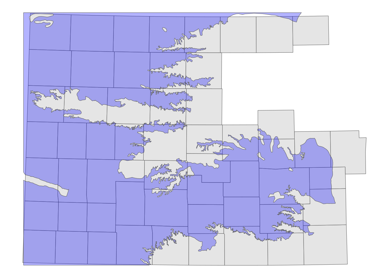
counties_intersecting_hpaSimple feature collection with 56 features and 9 fields
Geometry type: MULTIPOLYGON
Dimension: XY
Bounding box: xmin: 229253.5 ymin: 4094801 xmax: 690085.5 ymax: 4432561
Projected CRS: WGS 84 / UTM zone 14N
First 10 features:
STATEFP COUNTYFP COUNTYNS AFFGEOID GEOID NAME LSAD ALAND
2 20 075 00485327 0500000US20075 20075 Hamilton 06 2580958328
4 20 189 00485056 0500000US20189 20189 Stevens 06 1883595654
5 20 155 00485041 0500000US20155 20155 Reno 06 3251786677
6 20 129 00485135 0500000US20129 20129 Morton 06 1889994372
8 20 023 00484981 0500000US20023 20023 Cheyenne 06 2641501921
9 20 089 00485009 0500000US20089 20089 Jewell 06 2356813568
11 20 077 00485004 0500000US20077 20077 Harper 06 2075290355
14 20 165 00485358 0500000US20165 20165 Rush 06 1858997546
15 20 097 00485013 0500000US20097 20097 Kiowa 06 1871627782
16 20 109 00485019 0500000US20109 20109 Logan 06 2779039721
AWATER geometry
2 2893322 MULTIPOLYGON (((233615.1 42...
4 464936 MULTIPOLYGON (((273665.9 41...
5 42963060 MULTIPOLYGON (((546178.6 42...
6 507796 MULTIPOLYGON (((229431.1 41...
8 2738021 MULTIPOLYGON (((239494.1 44...
9 11367163 MULTIPOLYGON (((542298.2 44...
11 3899269 MULTIPOLYGON (((557559.9 41...
14 544720 MULTIPOLYGON (((449120.4 42...
15 596764 MULTIPOLYGON (((450693.8 41...
16 274632 MULTIPOLYGON (((285802.7 43...# sf_1[sf_2, op = topological_relation_type]KS_corn_price <-
KS_counties %>%
dplyr::mutate(corn_price = seq(3.2, 3.9, length = nrow(.))) %>%
dplyr::select(COUNTYFP, corn_price)
KS_corn_priceSimple feature collection with 105 features and 2 fields
Geometry type: MULTIPOLYGON
Dimension: XY
Bounding box: xmin: 229253.5 ymin: 4094801 xmax: 890007.5 ymax: 4434288
Projected CRS: WGS 84 / UTM zone 14N
First 10 features:
COUNTYFP corn_price geometry
1 133 3.200000 MULTIPOLYGON (((806203.1 41...
2 075 3.206731 MULTIPOLYGON (((233615.1 42...
3 123 3.213462 MULTIPOLYGON (((544031.7 43...
4 189 3.220192 MULTIPOLYGON (((273665.9 41...
5 155 3.226923 MULTIPOLYGON (((546178.6 42...
6 129 3.233654 MULTIPOLYGON (((229431.1 41...
7 073 3.240385 MULTIPOLYGON (((717254.1 42...
8 023 3.247115 MULTIPOLYGON (((239494.1 44...
9 089 3.253846 MULTIPOLYGON (((542298.2 44...
10 059 3.260577 MULTIPOLYGON (((804792.9 42...(
KS_wells_County <- sf::st_join(KS_wells, KS_corn_price)
)Simple feature collection with 37647 features and 4 fields
Geometry type: POINT
Dimension: XY
Bounding box: xmin: 230332 ymin: 4095052 xmax: 887329.7 ymax: 4433597
Projected CRS: WGS 84 / UTM zone 14N
First 10 features:
site af_used COUNTYFP corn_price geometry
1 1 232.099948 069 3.556731 POINT (372548 4153588)
2 3 13.183940 039 3.449038 POINT (353698.6 4419755)
3 5 99.187052 165 3.287500 POINT (486771.7 4260027)
4 7 0.000000 199 3.644231 POINT (248127.1 4296442)
5 8 145.520499 055 3.832692 POINT (349813.2 4215310)
6 9 3.614535 143 3.799038 POINT (612277.6 4322077)
7 11 188.423543 181 3.590385 POINT (267030.7 4381364)
8 12 77.335960 177 3.550000 POINT (761774.6 4339039)
9 15 0.000000 159 3.610577 POINT (560570.3 4235763)
10 17 167.819034 069 3.556731 POINT (387315.1 4175007)KS_wells %>% aggregate(KS_counties, FUN = sum)Simple feature collection with 105 features and 2 fields
Geometry type: MULTIPOLYGON
Dimension: XY
Bounding box: xmin: 229253.5 ymin: 4094801 xmax: 890007.5 ymax: 4434288
Projected CRS: WGS 84 / UTM zone 14N
First 10 features:
site af_used geometry
1 124453 1.701790e+01 MULTIPOLYGON (((806203.1 41...
2 12514550 6.261704e+04 MULTIPOLYGON (((233615.1 42...
3 1964254 1.737791e+03 MULTIPOLYGON (((544031.7 43...
4 42442400 3.023589e+05 MULTIPOLYGON (((273665.9 41...
5 68068173 6.110576e+04 MULTIPOLYGON (((546178.6 42...
6 15756801 9.664610e+04 MULTIPOLYGON (((229431.1 41...
7 149202 0.000000e+00 MULTIPOLYGON (((717254.1 42...
8 17167377 5.750807e+04 MULTIPOLYGON (((239494.1 44...
9 1809003 2.201696e+03 MULTIPOLYGON (((542298.2 44...
10 160064 4.571102e+00 MULTIPOLYGON (((804792.9 42...# sf::st_join(sf_1, sf_2, join = \(x, y) st_is_within_distance(x, y, dist = 5))
# st_intersection() => does cropped join