Geospatial with R

Practicing GIS in R

This is my practice sections following blog posts by Andrew Heiss.

Middle earth maps with R

Middle earth maps with R

Quick reminder: latitude vs. longitude

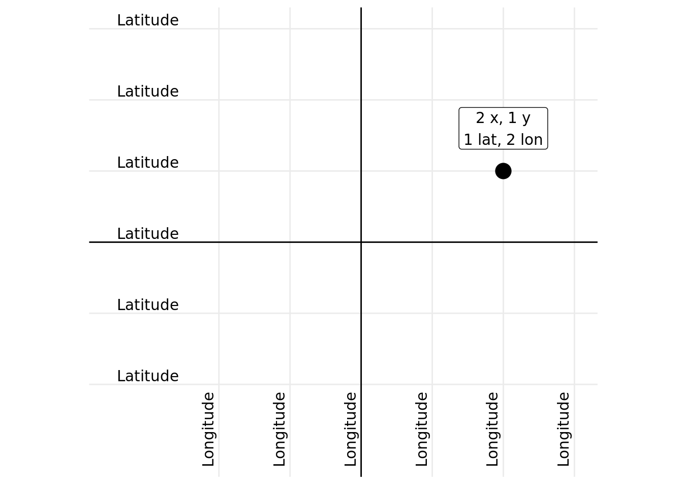
library(data.table)
library(tidyverse)
library(sf)
library(rnaturalearth)
library(scales)
library(patchwork)
library(leaflet)
library(glue)

point_example <- tibble(x = 2, y = 1) %>% 
  mutate(label = glue::glue("{x} x, {y} y\n{y} lat, {x} lon"))
lat_labs <- tibble(x = -3, y = seq(-2, 3, 1), label = "Latitude")
lon_labs <- tibble(x = seq(-2, 3, 1), y = -2, label = "Longitude")

ggplot() +
  geom_point(data = point_example, aes(x = x, y = y), size = 5) +
  geom_label(data = point_example, aes(x = x, y = y, label = label),
            nudge_y = 0.6, family = "Overpass ExtraBold") +
  geom_text(data = lat_labs, aes(x = x, y = y, label = label),
            hjust = 0.5, vjust = -0.3, family = "Overpass Light") +
  geom_text(data = lon_labs, aes(x = x, y = y, label = label),
            hjust = 1.1, vjust = -0.5, angle = 90, family = "Overpass Light") +
  geom_hline(yintercept = 0) +
  geom_vline(xintercept = 0) +
  scale_x_continuous(breaks = seq(-2, 3, 1)) +
  scale_y_continuous(breaks = seq(-2, 3, 1)) +
  coord_equal(xlim = c(-3.5, 3), ylim = c(-3, 3)) +
  labs(x = NULL, y = NULL) +
  theme_minimal() +
  theme(panel.grid.minor = element_blank(),
        axis.text = element_blank()) 

Start the middle earth mapping

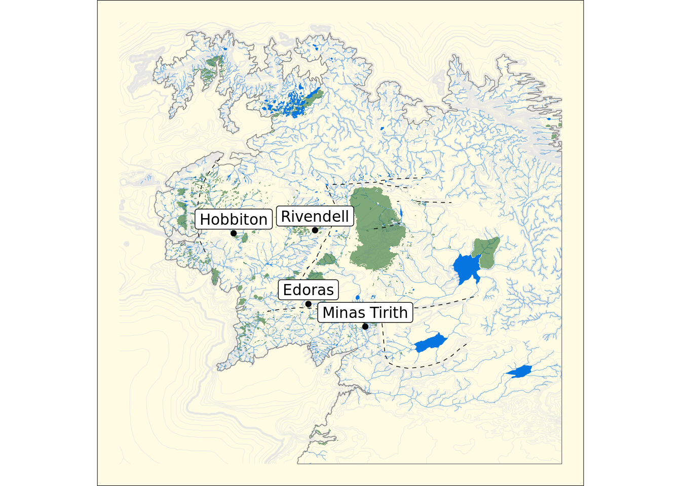
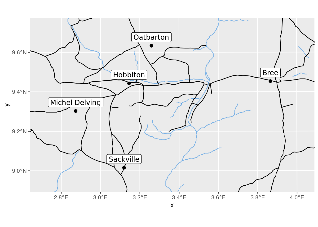
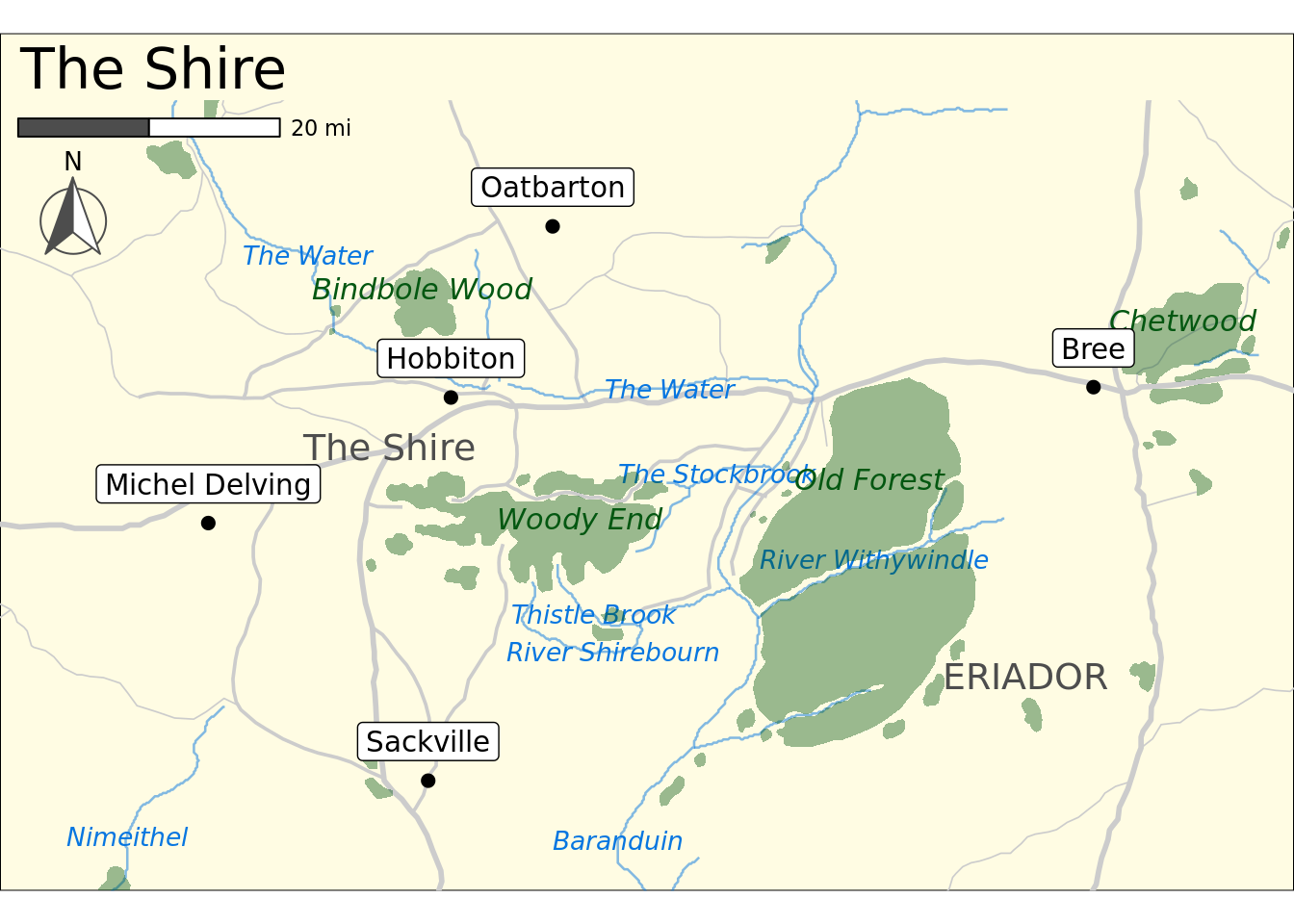
coastline <- read_sf("data/ME-GIS/Coastline2.shp") %>% 
  mutate(across(where(is.character), ~iconv(., from = "ISO-8859-1", to = "UTF-8")))

contours <- read_sf("data/ME-GIS/Contours_18.shp") %>% 
  mutate(across(where(is.character), ~iconv(., from = "ISO-8859-1", to = "UTF-8")))

rivers <- read_sf("data/ME-GIS/Rivers.shp") %>% 
  mutate(across(where(is.character), ~iconv(., from = "ISO-8859-1", to = "UTF-8")))

roads <- read_sf("data/ME-GIS/Roads.shp") %>% 
  mutate(across(where(is.character), ~iconv(., from = "ISO-8859-1", to = "UTF-8")))

lakes <- read_sf("data/ME-GIS/Lakes.shp") %>% 
  mutate(across(where(is.character), ~iconv(., from = "ISO-8859-1", to = "UTF-8")))

regions <- read_sf("data/ME-GIS/Regions_Anno.shp") %>% 
  mutate(across(where(is.character), ~iconv(., from = "ISO-8859-1", to = "UTF-8")))

forests <- read_sf("data/ME-GIS/Forests.shp") %>% 
  mutate(across(where(is.character), ~iconv(., from = "ISO-8859-1", to = "UTF-8")))

mountains <- read_sf("data/ME-GIS/Mountains_Anno.shp") %>% 
  mutate(across(where(is.character), ~iconv(., from = "ISO-8859-1", to = "UTF-8")))

placenames <- read_sf("data/ME-GIS/Combined_Placenames.shp") %>% 
  mutate(across(where(is.character), ~iconv(., from = "ISO-8859-1", to = "UTF-8")))

miles_to_meters <- function(x) {
  x * 1609.344
}

meters_to_miles <- function(x) {
  x / 1609.344
}

clr_green <- "#035711"
clr_blue <- "#0776e0"
clr_yellow <- "#fffce3"

# Format numeric coordinates with degree symbols and cardinal directions
format_coords <- function(coords) {
  ns <- ifelse(coords[[1]][2] > 0, "N", "S")
  ew <- ifelse(coords[[1]][1] > 0, "E", "W")
  
  glue("{latitude}°{ns} {longitude}°{ew}",
       latitude = sprintf("%.6f", coords[[1]][2]),
       longitude = sprintf("%.6f", coords[[1]][1]))
}

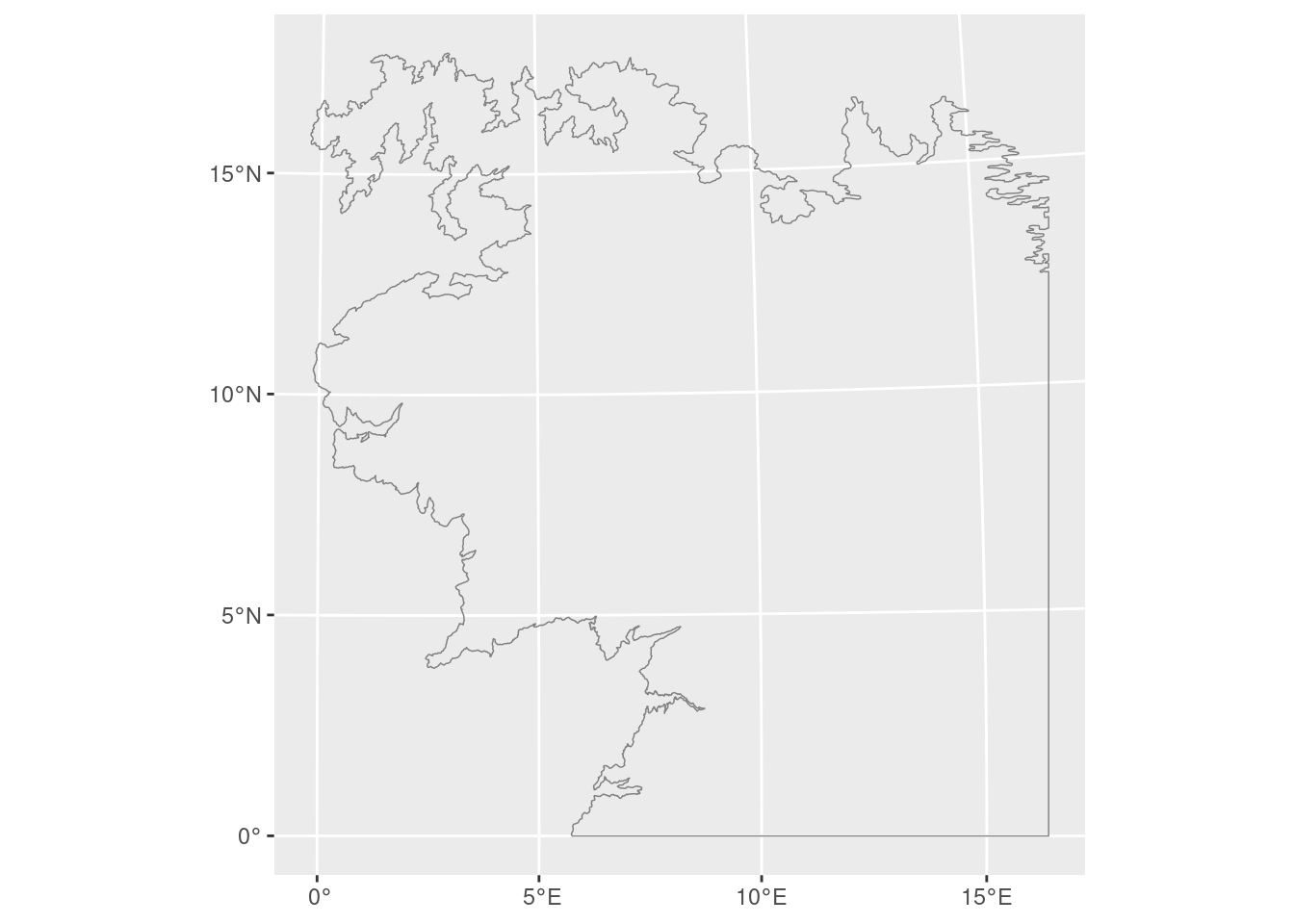
Exploring the different layers

ggplot() +
  geom_sf(data = coastline, linewidth = 0.25, color = "grey50")

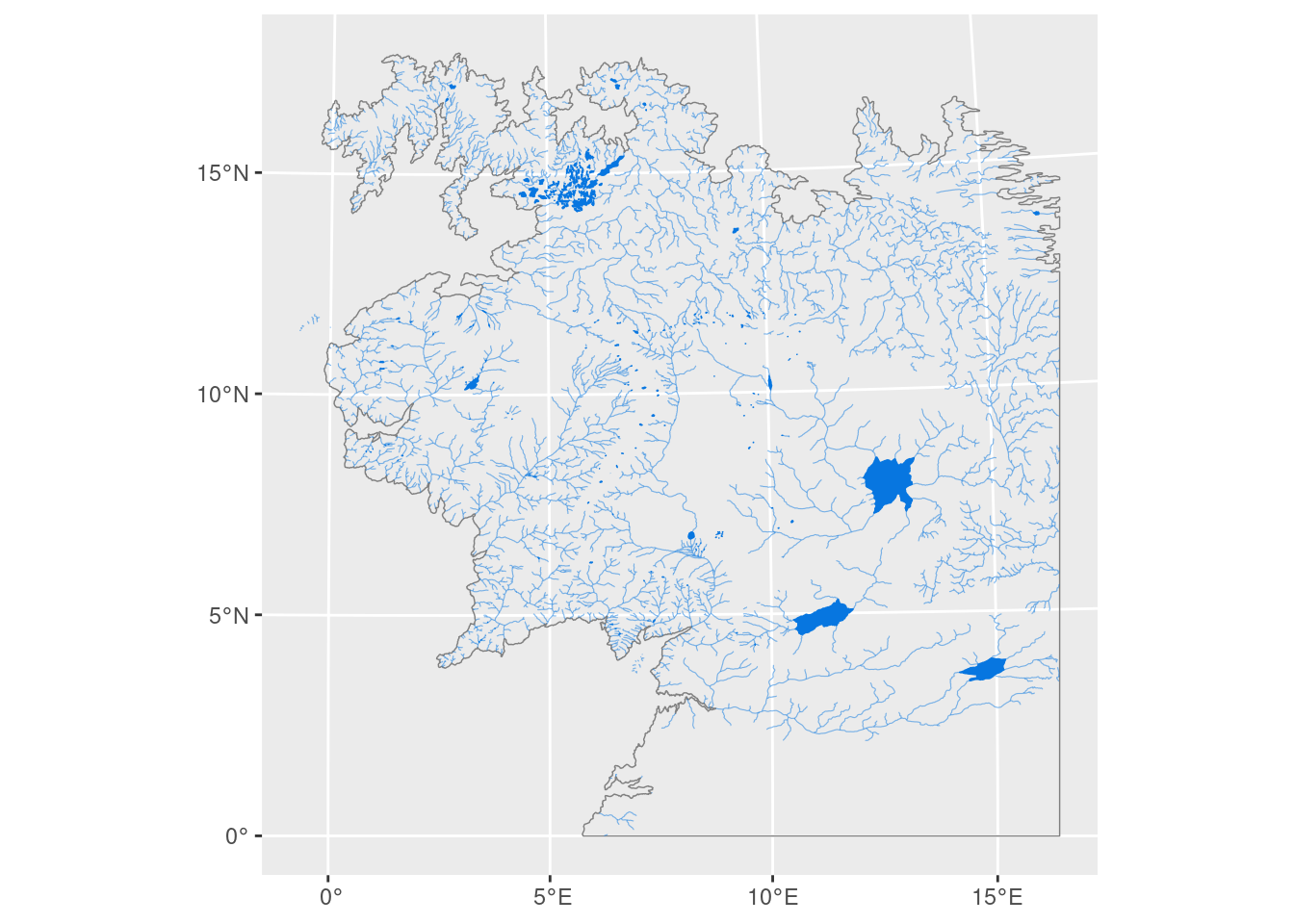
Add rivers and lakes

ggplot() +
  geom_sf(data = coastline, linewidth = 0.25, color = "grey50") +
  geom_sf(data = rivers, linewidth = 0.2, color = clr_blue, alpha = 0.5) +
  geom_sf(data = lakes, linewidth = 0.2, color = clr_blue, fill = clr_blue)

Putting some labels

places <- placenames %>% 
  filter(NAME %in% c("Hobbiton", "Rivendell", "Edoras", "Minas Tirith"))

ggplot()+
  geom_sf(data = coastline, linewidth = 0.25, color = "grey50") +
  geom_sf(data = rivers, linewidth = 0.2, color = clr_blue, alpha = 0.5) +
  geom_sf(data = lakes, linewidth = 0.2, color = clr_blue, fill = clr_blue) +
  geom_sf(data = places, size = 1) +
  geom_sf_label(data = places, aes(label = NAME), nudge_y = miles_to_meters(50))

Fancy map with lot of layers

places <- placenames %>% 
  filter(NAME %in% c("Hobbiton", "Rivendell", "Edoras", "Minas Tirith"))

ggplot() +
  geom_sf(data = contours, linewidth = 0.15, color = "grey90") +
  geom_sf(data = coastline, linewidth = 0.25, color = "grey50") +
  geom_sf(data = rivers, linewidth = 0.2, color = clr_blue, alpha = 0.5) +
  geom_sf(data = lakes, linewidth = 0.2, color = clr_blue, fill = clr_blue) +
  geom_sf(data = forests, linewidth = 0, fill = clr_green, alpha = 0.5) +
  geom_sf(data = mountains, linewidth = 0.25, linetype = "dashed") +
  geom_sf(data = places) +
  geom_sf_label(data = places, aes(label = NAME), nudge_y = miles_to_meters(40),
                family = "Overpass ExtraBold", fontface = "plain") +
  theme_void() +
  theme(plot.background = element_rect(fill = clr_yellow))

Focusing on Shire

hobbiton <- places %>% 
  filter(NAME == "Hobbiton") %>% 
  mutate(geometry_x = map_dbl(geometry, ~as.numeric(.)[1]),
         geometry_y = map_dbl(geometry, ~as.numeric(.)[2]))

hobbiton %>% 
  select(LAYER, NAME, geometry_x, geometry_y)

Simple feature collection with 1 feature and 4 fields
Geometry type: POINT
Dimension:     XY
Bounding box:  xmin: 515948 ymin: 1043820 xmax: 515948 ymax: 1043820
Projected CRS: UTM_Zone_31_Northern_Hemisphere
# A tibble: 1 × 5
  LAYER     NAME     geometry_x geometry_y         geometry
  <chr>     <chr>         <dbl>      <dbl>      <POINT [m]>
1 TownNames Hobbiton    515948.   1043820. (515948 1043820)

shire_towns <- placenames %>% filter(LAYER == "TownNames")

ggplot() +
  geom_sf(data = rivers, linewidth = 0.45, color = clr_blue, alpha = 0.5) +
  geom_sf(data = roads) +
  geom_sf(data = shire_towns, size = 2) +
  geom_sf_label(data = shire_towns, aes(label = NAME), nudge_y = miles_to_meters(3),
                family = "Overpass ExtraBold", fontface = "plain") +
  coord_sf(xlim = c(hobbiton$geometry_x - miles_to_meters(30), 
                    hobbiton$geometry_x + miles_to_meters(60)),
           ylim = c(hobbiton$geometry_y - miles_to_meters(35), 
                    hobbiton$geometry_y + miles_to_meters(20)))

Fancy map of Shire

library(ggspatial) 

shire_towns <- placenames %>% filter(LAYER == "TownNames")

ggplot() +
  geom_sf(data = roads, aes(linewidth = TYPE), color = "grey80") +
  geom_sf(data = coastline, linewidth = 0.25, color = "grey50") +
  geom_sf(data = rivers, linewidth = 0.45, color = clr_blue, alpha = 0.5) +
  geom_sf_text(data = rivers, aes(label = NAME), color = clr_blue,
               family = "Overpass SemiBold", fontface = "italic", size = 3.5) +
  geom_sf_text(data = regions, aes(label = name),
               family = "Overpass Heavy", size = 5, color = "grey30") +
  geom_sf(data = forests, linewidth = 0, fill = clr_green, alpha = 0.4) +
  geom_sf_text(data = forests, aes(label = NAME), nudge_y = miles_to_meters(1),
               color = clr_green, family = "Overpass ExtraBold", fontface = "italic", size = 4) +
  geom_sf(data = shire_towns, size = 2) +
  geom_sf_label(data = shire_towns, aes(label = NAME), nudge_y = miles_to_meters(3),
                family = "Overpass ExtraBold", fontface = "plain") +
  scale_linewidth_discrete(range = c(1, 0.3), guide = "none") +
  annotation_scale(location = "tl", bar_cols = c("grey30", "white"),
                   text_family = "Overpass",
                   unit_category = "imperial") +
  annotation_north_arrow(
    location = "tl", pad_y = unit(1.5, "lines"),
    style = north_arrow_fancy_orienteering(fill = c("grey30", "white"), 
                                           line_col = "grey30",
                                           text_family = "Overpass")) +
  coord_sf(xlim = c(hobbiton$geometry_x - miles_to_meters(30), 
                    hobbiton$geometry_x + miles_to_meters(60)),
           ylim = c(hobbiton$geometry_y - miles_to_meters(35), 
                    hobbiton$geometry_y + miles_to_meters(20))) +
  labs(title = "The Shire") +
  theme_void() +
  theme(plot.background = element_rect(fill = clr_yellow),
        plot.title = element_text(family = "Aniron", size = rel(2), 
                                  hjust = 0.02))

Distances between places

rivendell <- places %>% filter(NAME == "Rivendell")

st_distance(hobbiton, rivendell) %>% meters_to_miles()

Units: [m]
         [,1]
[1,] 229.0673

How to use a histogram as a legend in {ggplot2}

Cite: link